
As part of an initial pilot study off the California coast, in the upwelling-rich California Current System, off the coast of San Luis Obispo Bay (SLO Bay), researchers from the Virginia Institute of Marine Science (VIMS) along with scientists from MLML, Cal Poly San Luis Obispo and UC Santa Cruz, used an
Acoustic Doppler Current Profiler (ADCP) manufactured by
Teledyne RDI to make key velocity measurements to understand the dynamics of a submesoscale front in a coastal upwelling system, as part of a multi-institutional NSF funded project.
Researchers measured current velocities concurrently with other variables, such as temperature, salinity, dissolved oxygen, chl, surface nitrate, and turbulence, to provide a baseline map of the domain (spatial extent) and associated structure and trajectory of a key nearshore thermal front.
ADCP-derived circulation measurements depict the crucial internal and coastal exchange and processes related to physical circulation dynamics – particularly in areas where upwelling-generated dynamics have relatively strong control on local ecosystem processes.
Studying Submesoscale Fronts and Cross-Shelf Exchange
 SLO Bay, in the eastern boundary upwelling system (EBUS), exhibits seasonally persistent thermal fronts along most of the mouth of the bay. This bottom topography drives much of the critical small-scale bay-ocean exchanges of nutrients, as well as seasonal local hypoxia (or low oxygen) and harmful algal blooms (HABs). Conventional models of these dynamics typically ignore submesoscale interactions likely to affect coastal ecology. Scientists are working on this multi-phase project to understand how submesoscale fronts affect coastal-ocean exchanges and the storage of organic and nutrient matter in the bay.
Role of Teledyne RDI ADCP Technology
The
ADCP, produced by
Teledyne RDI, was lowered to the bottom of the sea to sample vertical velocity profiles that were then used to map the spatial and temporal circulation patterns of stretches of the SLO Bay current. One goal was to learn how these waters move through fronts – thin and highly mobile barriers between adjacent waters – and how to capture them. The
ADCP provided accurate, high-resolution readings of spatial frontal scales. This allowed for submesoscale features that could lead to a better understanding of cumulative exchange processes throughout the entire bay.
The pole-mounted ADCP provides current velocity readings that can be placed within the anywhere, anytime spatial context of all the other data acquired – temperature, turbulence, sound velocity, etc. The result is a series of multi-dimensional datasets essential to creating a ‘circulation map’ of how water moves around – and out of – SLO Bay, both seasonally and at tidal time.

Data Insights and Future Applications
In the meantime, while data processing is in progress, preliminary results should reveal just how much water circulates within and beyond the bay during different seasons. The ADCP velocity data can be combined with high-resolution subsurface measurements of temperature and turbulence to reveal a detailed picture of the submesoscale processes involved and how these fronts control nutrient and particulate retention, dispersion, and exchange. The data collected could also serve as a basis for more intensive field studies planned for the following years, involving a denser mooring array and more advanced ship-based surveys to explore these turbulent interactions in greater detail.
Broader Implications
 The results could change how we think about climate impacts, hypoxia, and harmful algal bloom formation in upwelling bays and managing these small embayments as sentinel environments. Knowing how SLO Bay is circulated will inform future coastal management of risk factors for marine life and ecosystem health.
“Using Teledyne RDI’s ADCP technology has been transformative in our study of submesoscale fronts in SLO Bay. The high-resolution velocity measurements allow us to capture detailed circulation patterns critical for understanding nutrient dynamics and ecosystem health in this coastal upwelling system. With the ADCP, we can map currents and fronts with unprecedented precision, providing insights crucial for future coastal management and ecosystem preservation,” said Piero Mazzini, Coastal Physical Oceanographer at VIMS.
ADCP technology in this project demonstrates how combining high-resolution, near-real-time ADCP data with interdisciplinary research methods allows researchers to approach complex environmental questions. Teledynes RDI’s ADCP technology opens up the potential to fill an age-old gap between oceanographic models and measured data to understand small-scale oceanographic processes further. The results of this pilot in SLO Bay will be applied in future studies to protect our coastal ecosystems better while the ocean keeps getting warmer.
Example of Data
VIMS collected a 2,700 meter long vessel survey transect in the north east direction (course made good = 35 degrees). Figure 1 depicts the ship track as the Red Line with the blue vectors corresponding to the current speed and direction. At a depth of 2.2 meters we see that the currents are flowing to the direction of the vector. At the beginning of the transect the currents were generally flowing to the south-east and at a distance of ~700 meters to the east and 1000 meters to the north, the vessel passes into another flow regime where the currents are generally flowing to the west - south west.
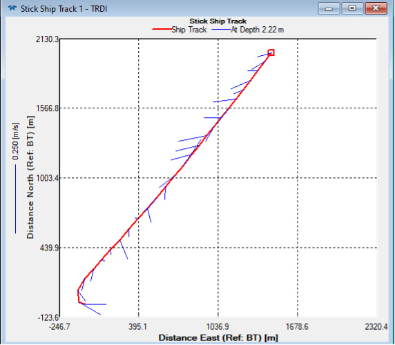
Figure 1: Stick Ship Track – Currents at 2.2 m depth with >90 degree changes in current direction in the middle of the transect.
|  Figure 2: Stick Ship Track – Currents at 10.2 m depth with currents generally flowing to the west north west along the entire transect. Figure 2: Stick Ship Track – Currents at 10.2 m depth with currents generally flowing to the west north west along the entire transect.
|

Figure 3: Plot of the vertical variation of the velocity direction across the length of the transect with near surface currents directed to the north east (blue) with an abrupt vertical shear at a depth of 10 meters with the deeper currents north west (Red) near the bottom at the beginning of the transect and a frontal boundary at a length of ~1700 meters in the transect where the water column is well mixed and flowing to the north west.

